14 Quantile Regression (+)
Lona Koers
Ludwig-Maximilians-Universität München
14.1 Introduction
Regression models typically predict the conditional mean of the target given the input features. Quantile regression allows predicting conditional quantiles, enabling more uncertainty-aware and informative predictions or an approximation of the conditional distribution. Instead of answering “What is the expected outcome given these features?”, quantile regression asks, “What is the outcome at a given probability level (e.g., 10th percentile, median, 90th percentile)?”.
This is particularly useful in scenarios where we want to model uncertainty and extremes in data:
- Constructing prediction intervals, by asking for a lower bound, a central prediction, and an upper bound (e.g. 0.05, 0.5, or 0.95)
- Identifying extreme values: In applications such as risk analysis, financial modeling, or weather forecasting, we may be particularly interested in predicting the worst-case or best-case outcomes (e.g., the 5th quantile for a stock price drop).
- Handling heteroscedastic data: When the variance of the response variable changes with the input features, quantile regression is usually a more robust solution.
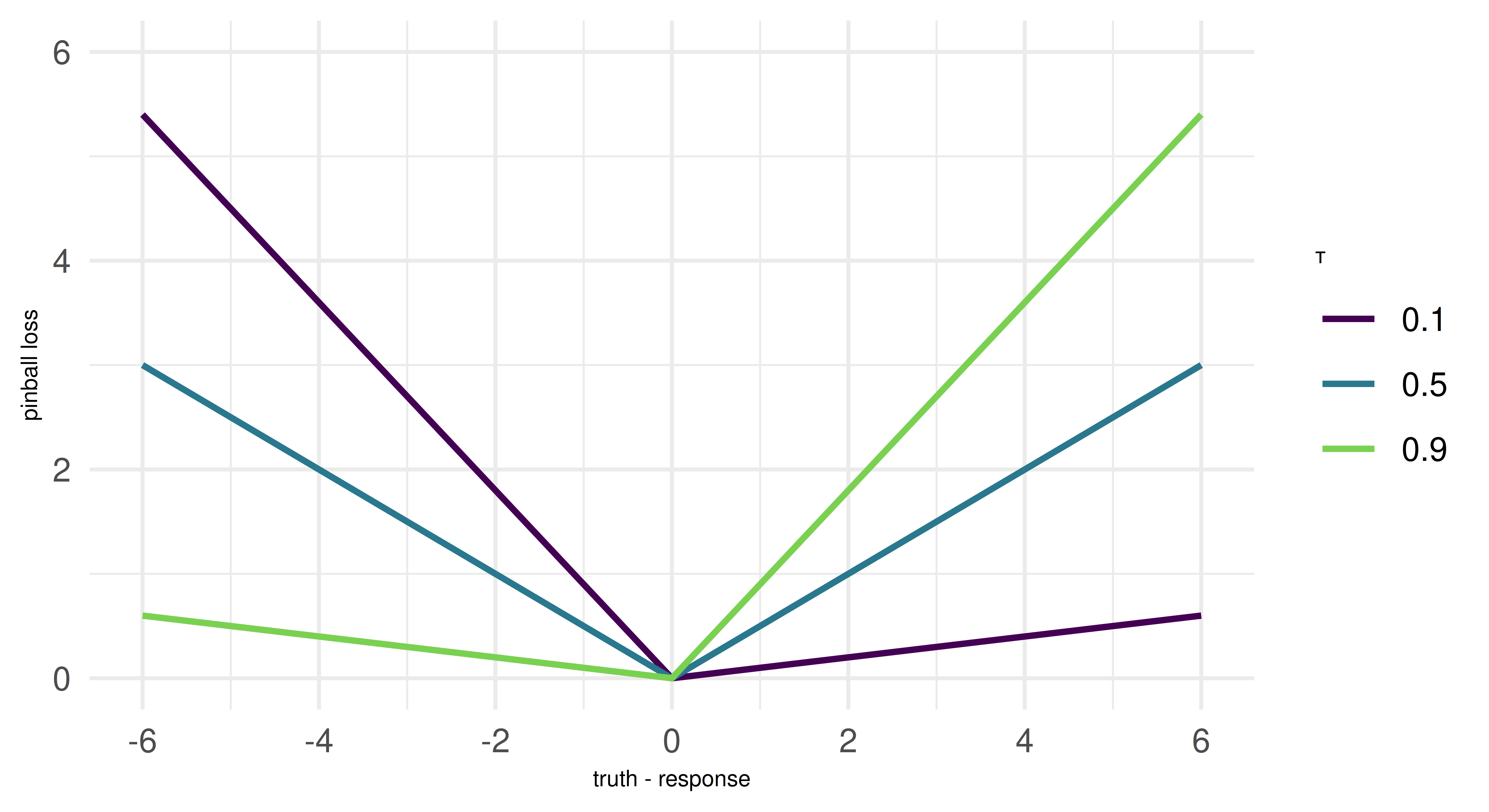
A key concept in estimating quantile regression models is the pinball loss, which generalizes the L1 loss, or mean absolute error (MAE), to optimize for arbitrary quantiles \(\tau\). To understand this, we need to recall that the median (i.e. the 0.5-quantile) minimizes the MAE. The pinball loss modifies the L1 loss by introducing an asymmetry that encourages the model to penalize under- or over-prediction more heavily, based on the chosen quantile level. For instance, setting \(\tau = 0.1\) means overpredictions are nine times more expensive than underpredictions, leading the model to systematically underestimate the target. This pushes the model to estimate not the center of the (conditional) distribution, but the selected quantile. We can connect this directly to quantiles: If the model is trained to minimize pinball loss for a given quantile \(\tau\), then \(\tau \%\) of the observed values should be below the predicted value, and \((1 - \tau) \%\) should be above it. For example, a model trained with \(\tau = 0.1\) will produce predictions such that 10% of observed values fall below its predictions, making it an estimator of the 10th percentile. The pinball loss will reappear as an evaluation metric at the end of this chapter.
But note: While many ML models based on empirical risk minimization use the pinball loss for estimating quantiles, some model classes might work differently. But since the undelying training procedure of a model is external to mlr3, we are more concerned with resampling and evaluating quantile regression models. This works in exactly the same manner as for other tasks. Because we provieded only a brief overview over quantile regression, we recommend Yu, Lu, and Stander (2003) if you are interested in a methodological introduction into the topic.
14.2 Synthetic data set generation
Let’s construct a simple synthetic data set to demonstrate how quantile regression works.
We generate 10,000 data points where the univariate feature x is drawn from a uniform distribution between 1 and 15 and the target y follows a non-linear function of x. To make the problem more interesting, we use heteroskedastic Gaussian noise on the target, i.e. the variance increases as x increases.
Let’s plot the data to get a better feel for it. The points are a random subset of the data (10%). The line is the true underlying function \(f(x)\), from which we sampled and which we would ideally recover as our estimated posterior median.
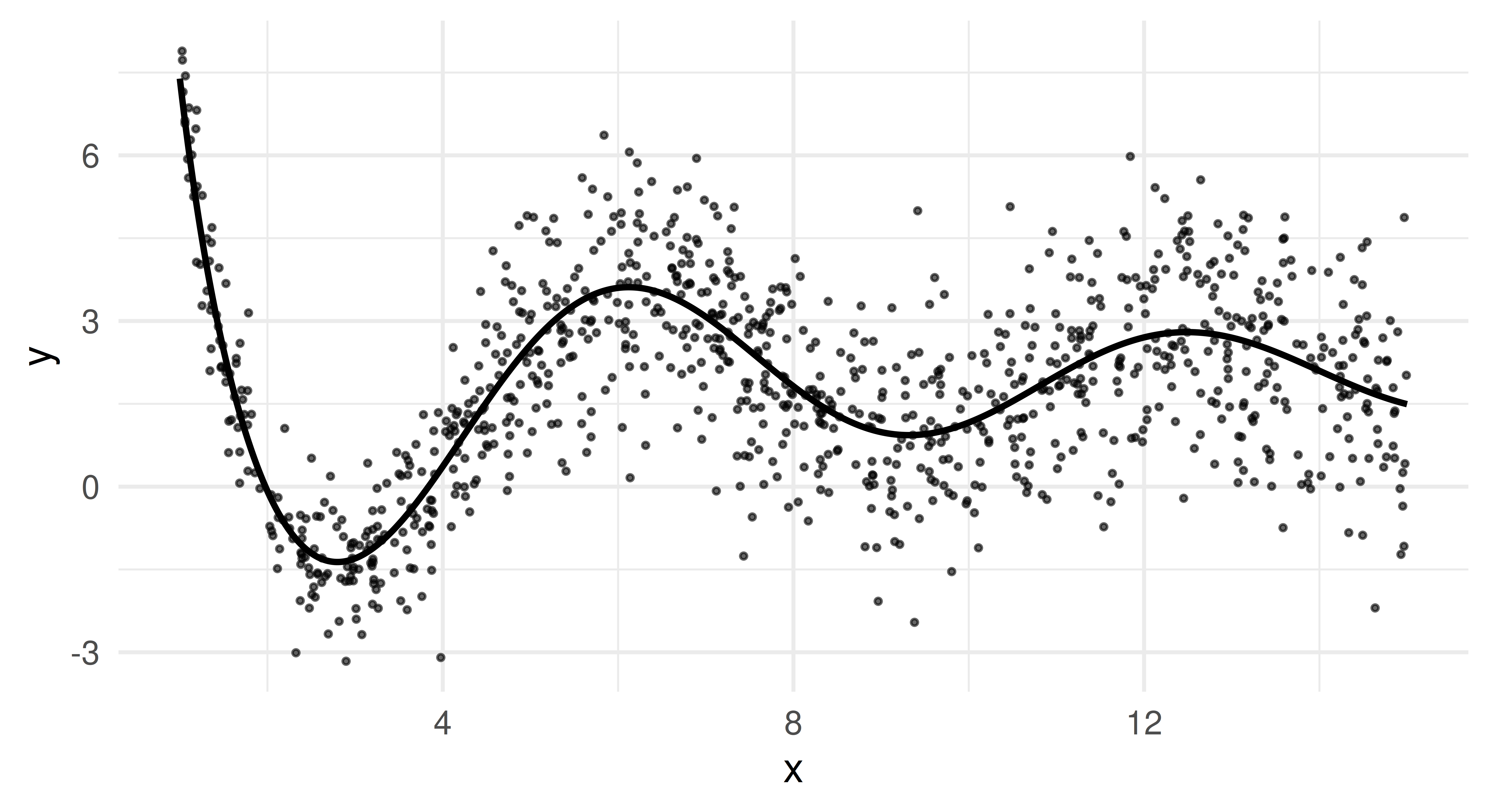
This plot reveals two essential properties of our data. Firstly, \(f(x)\) oscillates more for small x but becomes smoother for larger values. Secondly, we clearly see heteroscedasticity as the variance of y increases as x grows.
Because of the latter, mean-based models will struggle to provide robust predictions, especially for larger values of x, as they will be heavily influenced by extreme deviations. In contrast, the median (0.5-quantile) provides a more stable estimate, while other quantiles (e.g., 0.05 and 0.95) allow us to estimate uncertainty and extreme outcomes.
Now that we have generated our data set, we transform it into a regular regression task and split it into a train and test set. We also specify five quantiles to estimate. The median, which we will soon set as the intended response and four other quantiles to to capture lower and upper dispersion.
library(mlr3verse)

task = as_task_regr(data, target = "y")
splits = partition(task)

qs = c(0.05, 0.25, 0.5, 0.75, 0.95)
14.3 Quantile Regression with Multiple Learners
14.3.1 Random Regression Forest
The first learner we apply is a random regression forest (lrn("regr.ranger")), implemented in mlr3learners, a tree-based ensemble which can nicely handle complex interactions and non-linear relationships. We configure the learner to predict the specified quantiles and mark the median quantile as the dedicated response. We then train and predict as usual.
lrn_ranger = lrn("regr.ranger", predict_type = "quantiles",
                     quantiles = qs, quantile_response = 0.5)
lrn_ranger$param_set$set_values(min.node.size = 10, num.trees = 100, mtry = 1)
lrn_ranger$train(task, row_ids = splits$train)

prds_ranger = lrn_ranger$predict(task, row_ids = splits$test)
prds_ranger
── <PredictionRegr> for 3300 observations: ──────────────────────────────
 row_ids  truth   q0.05   q0.25      q0.5  q0.75 q0.95  response
       7 2.0796 -1.3721 -0.7666  0.542457 3.3556 3.920  0.542457
      10 2.2017 -0.9629 -0.9629  0.006732 1.9025 3.187  0.006732
      11 0.9907  0.7899  2.2841  2.368496 3.7757 5.561  2.368496
     ---    ---     ---     ---       ---    ---   ---       ---
    9988 0.7872  0.4666  0.8145  1.540437 1.9588 2.627  1.540437
    9997 3.7753 -0.7441 -0.7441  1.159466 3.3396 4.482  1.159466
    9999 2.1826 -2.3695 -1.1470 -0.094602 0.4536 2.236 -0.094602
The predict object has additional columns for all quantiles. We set $quantile_response = 0.5 which means that response is equal to the 0.5-quantile.
We now plot the predicted quantiles against the true test data. Each colored line represents a different quantile estimate, and the black curve represents the true function.
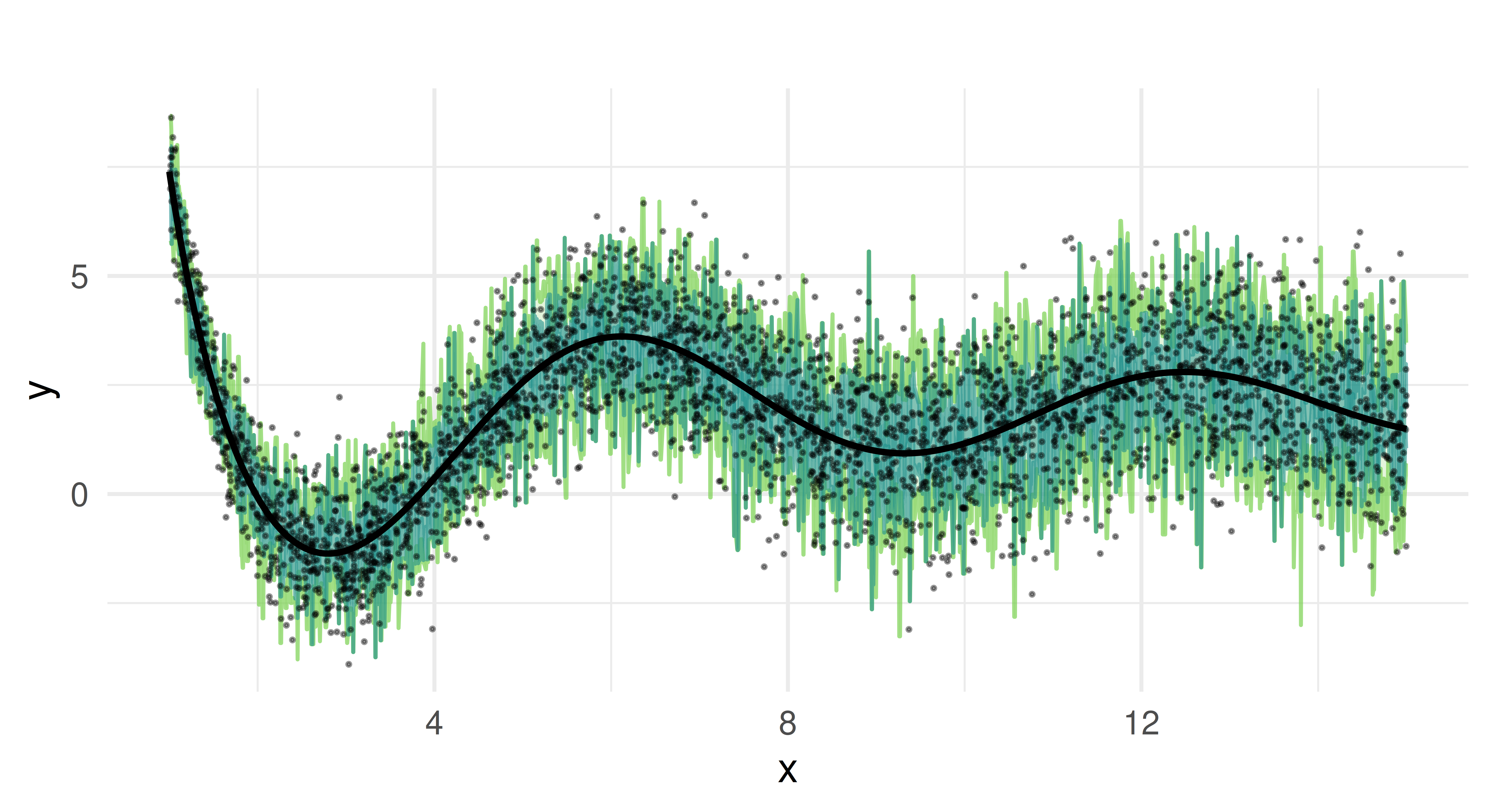
We can see that the random forest captures the overall trend of the function. It provides quantile estimates that increase as x increases and handles the non-linearity of our data well due to its ensemble nature.
But the predicted quantiles appear overly jagged and spiky, which suggests that the model might be overfitting to the noise in the training data rather than capturing smooth trends. The median estimate oscillates around the true function but does not consistently align with it. The reason for these limitations lies in how random forests construct quantiles. In quantile regression forests, predictions are derived from the empirical distribution of the response values within the terminal nodes of individual trees. Each tree partitions the feature space into regions, and all observations that fall into the same region (terminal node) share the same conditional distribution estimate. Quantiles are computed based on the sorted values of these observations. Because the number of samples in each terminal node is finite, the estimated quantiles are discrete rather than continuous, leading to the characteristic “stair-step” appearance in the predictions. If a particular terminal node contains only a small number of observations, the estimated quantiles may shift abruptly between adjacent nodes, creating jagged or spiky predictions. Additionally, the aggregation across trees averages over multiple step functions, which can result in piecewise-constant and noisy quantile estimates.
14.3.2 Smooth Additive Model with PipeOpLearnerQuantiles
To address the limitations that we observed with the random regression forest, we will now consider quantile regression with smooth generalized additive models (GAM) as an alternative method. This approach allows for smoother estimates and may improve the robustness of quantile predictions. Unlike tree-based methods, GAMs construct their prediction function using smooth splines rather than discrete splits. This makes them well-suited for handling continuous and structured data – which here aligns here well with our simulation setup, although, in a more realistic scencario, we would not know this.
The predictive intervals we obtain from the quantile GAM differ from conventional confidence intervals in GAMs: rather than quantifying uncertainty around the estimated function itself, our quantile estimates enable direct predictive inference. This allows us to construct observation-wise prediction intervals.
We will begin to demonstrate this using lrn("regr.mqgam") from mlr3extralearners. As we have done above for the random regression forest, we fit a model using the previously specified quantiles.
library(mlr3extralearners)

lrn_mqgam = lrn("regr.mqgam", predict_type = "quantiles",
                quantiles = qs, quantile_response = 0.5)
lrn_mqgam$param_set$values$form = y ~ s(x)
lrn_mqgam$train(task, row_ids = splits$train)
Warning in newton(lsp = lsp, X = G$X, y = G$y, Eb = G$Eb, UrS = G$UrS, L
= G$L, : Fitting terminated with step failure - check results carefully
Warning in newton(lsp = lsp, X = G$X, y = G$y, Eb = G$Eb, UrS = G$UrS, L
= G$L, : Fitting terminated with step failure - check results carefully
Warning in newton(lsp = lsp, X = G$X, y = G$y, Eb = G$Eb, UrS = G$UrS, L
= G$L, : Fitting terminated with step failure - check results carefullyprds_mqgam = lrn_mqgam$predict(task, row_ids = splits$test)After training, we generate predictions for the test set and visualize the results.
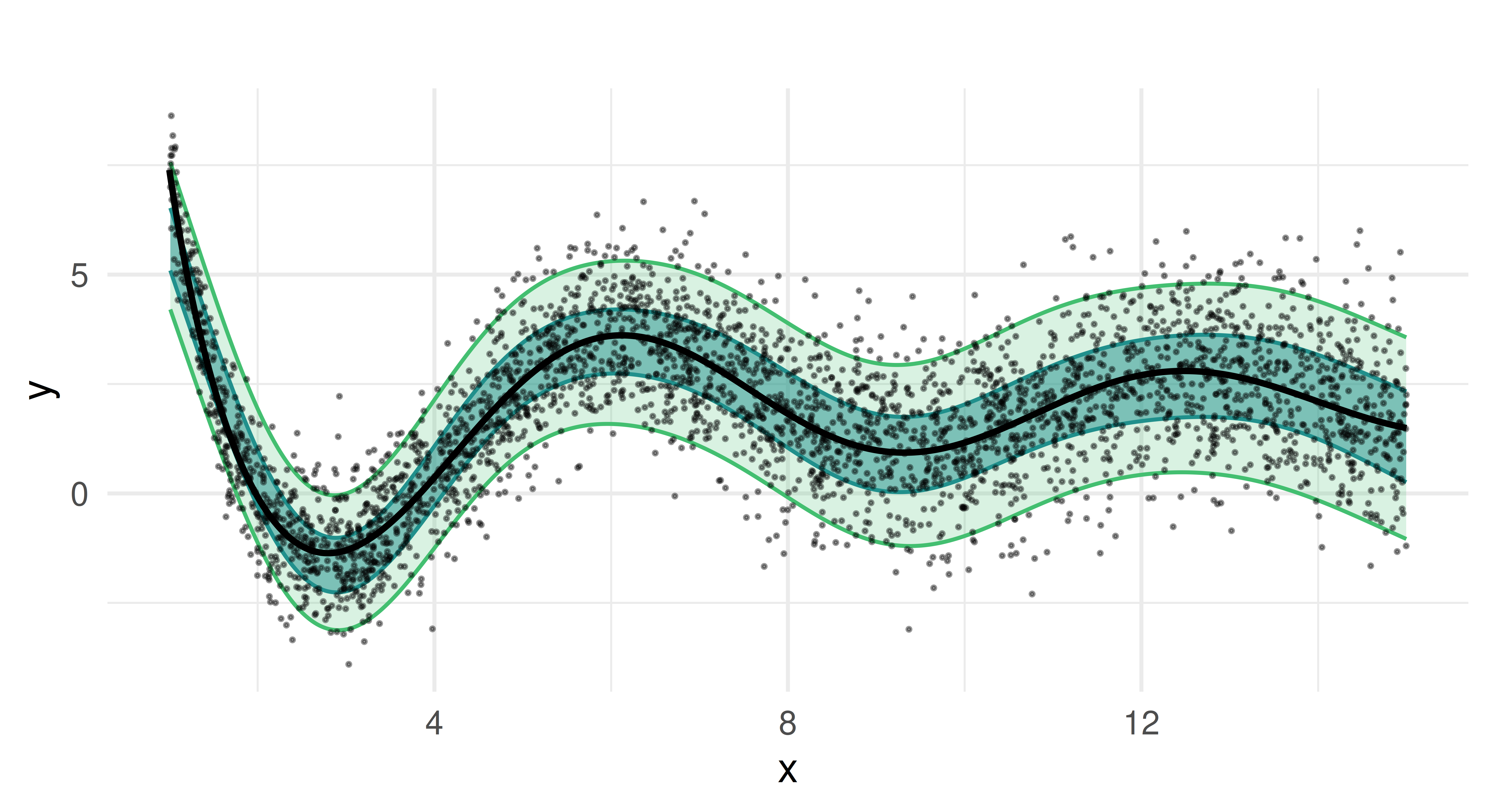
Compared to the random regression forest, the quantile GAM produces smoother estimates, as expected from an additive model. The predicted median closely follows the true function, and the estimated prediction intervals capture the heteroscedastic variance of the target well. Notably, the coverage of the quantiles is more stable, without the fluctuations seen in the random forest approach.
There are multiple learners in the mlr3verse which can’t predict multiple quantiles simultaneously. Because of this, we are also going to show how to use the po("learner_quantiles") from mlr3pipelines, which wraps a learner and extends its functionality to handle multiple quantiles in one step. Chapter 7 and Chapter 8 have already given an introduction to mlr3pipelines. We use this pipeop with lrn("regr.qgam"), a quantile regression GAM learner that can only be trained on one quantile.
We can then use GraphLearner to predict for the test set.
graph_lrn_qgam = as_learner(po_qgam)
graph_lrn_qgam$train(task, row_ids = splits$train)Warning in newton(lsp = lsp, X = G$X, y = G$y, Eb = G$Eb, UrS = G$UrS, L = G$L, : Fitting terminated with step failure - check results carefully
This happened PipeOp regr.qgam's $train()
Warning in newton(lsp = lsp, X = G$X, y = G$y, Eb = G$Eb, UrS = G$UrS, L = G$L, : Fitting terminated with step failure - check results carefully
This happened PipeOp regr.qgam's $train()prds_qgam = graph_lrn_qgam$predict(task, row_ids = splits$test)14.3.3 Comparison of methods
So far, we have only looked at a visualization of the predictions on the test data. We will now evaluate and benchmark the two models.
To evaluate how well each model predicts quantiles on our test data, we compute the pinball loss. In general, a lower absolute pinball loss indicates better accuracy for a given quantile alpha. Since extreme quantiles (e.g. 0.05 or 0.95) represent rare events and rely on less data for estimation, we would typically expect them to have higher loss than the median.
measures = list(msr("regr.pinball", alpha = 0.05, id = "q0.05"),
msr("regr.pinball", alpha = 0.25, id = "q0.25"),
msr("regr.pinball", alpha = 0.5, id = "q0.5"),
msr("regr.pinball", alpha = 0.75, id = "q0.75"),
msr("regr.pinball", alpha = 0.95, id = "q0.95"))
prds_ranger$score(measures) q0.05 q0.25 q0.5 q0.75 q0.95
0.1588 0.4295 0.5272 0.4188 0.1570 prds_mqgam$score(measures) q0.05 q0.25 q0.5 q0.75 q0.95
0.1236 0.3746 0.4703 0.3753 0.1228 In this case, the loss for more extreme quantiles is lower than that of the median. The quantiles modeled with the GAM provide a better fit than the random forest. This aligns with our previous results, where the GAM produced smoother quantile estimates than the random forest.
To further assess the quality of our models, we resample and benchmark the models with 10-fold cross validation. After resampling, the results can then aggregated and scored. This works as established in Chapter 3.
cv10 = rsmp("cv", folds = 10)
cv10$instantiate(task)
rr_ranger = resample(task, lrn_ranger, cv10)
rr_mqgam = resample(task, lrn_mqgam, cv10)Warning in newton(lsp = lsp, X = G$X, y = G$y, Eb = G$Eb, UrS = G$UrS, L
= G$L, : Fitting terminated with step failure - check results carefully
Warning in newton(lsp = lsp, X = G$X, y = G$y, Eb = G$Eb, UrS = G$UrS, L
= G$L, : Fitting terminated with step failure - check results carefully
Warning in newton(lsp = lsp, X = G$X, y = G$y, Eb = G$Eb, UrS = G$UrS, L
= G$L, : Fitting terminated with step failure - check results carefully
Warning in newton(lsp = lsp, X = G$X, y = G$y, Eb = G$Eb, UrS = G$UrS, L
= G$L, : Fitting terminated with step failure - check results carefully
Warning in newton(lsp = lsp, X = G$X, y = G$y, Eb = G$Eb, UrS = G$UrS, L
= G$L, : Fitting terminated with step failure - check results carefully
Warning in newton(lsp = lsp, X = G$X, y = G$y, Eb = G$Eb, UrS = G$UrS, L
= G$L, : Fitting terminated with step failure - check results carefully
Warning in newton(lsp = lsp, X = G$X, y = G$y, Eb = G$Eb, UrS = G$UrS, L
= G$L, : Fitting terminated with step failure - check results carefully
Warning in newton(lsp = lsp, X = G$X, y = G$y, Eb = G$Eb, UrS = G$UrS, L
= G$L, : Fitting terminated with step failure - check results carefully
Warning in newton(lsp = lsp, X = G$X, y = G$y, Eb = G$Eb, UrS = G$UrS, L
= G$L, : Fitting terminated with step failure - check results carefully
Warning in newton(lsp = lsp, X = G$X, y = G$y, Eb = G$Eb, UrS = G$UrS, L
= G$L, : Fitting terminated with step failure - check results carefully
Warning in newton(lsp = lsp, X = G$X, y = G$y, Eb = G$Eb, UrS = G$UrS, L
= G$L, : Fitting terminated with step failure - check results carefully
Warning in newton(lsp = lsp, X = G$X, y = G$y, Eb = G$Eb, UrS = G$UrS, L
= G$L, : Fitting terminated with step failure - check results carefully
Warning in newton(lsp = lsp, X = G$X, y = G$y, Eb = G$Eb, UrS = G$UrS, L
= G$L, : Fitting terminated with step failure - check results carefully
Warning in newton(lsp = lsp, X = G$X, y = G$y, Eb = G$Eb, UrS = G$UrS, L
= G$L, : Fitting terminated with step failure - check results carefully
Warning in newton(lsp = lsp, X = G$X, y = G$y, Eb = G$Eb, UrS = G$UrS, L
= G$L, : Fitting terminated with step failure - check results carefully
Warning in newton(lsp = lsp, X = G$X, y = G$y, Eb = G$Eb, UrS = G$UrS, L
= G$L, : Fitting terminated with step failure - check results carefully
Warning in newton(lsp = lsp, X = G$X, y = G$y, Eb = G$Eb, UrS = G$UrS, L
= G$L, : Fitting terminated with step failure - check results carefully
Warning in newton(lsp = lsp, X = G$X, y = G$y, Eb = G$Eb, UrS = G$UrS, L
= G$L, : Fitting terminated with step failure - check results carefully
Warning in newton(lsp = lsp, X = G$X, y = G$y, Eb = G$Eb, UrS = G$UrS, L
= G$L, : Fitting terminated with step failure - check results carefully
Warning in newton(lsp = lsp, X = G$X, y = G$y, Eb = G$Eb, UrS = G$UrS, L
= G$L, : Fitting terminated with step failure - check results carefully
Warning in newton(lsp = lsp, X = G$X, y = G$y, Eb = G$Eb, UrS = G$UrS, L
= G$L, : Fitting terminated with step failure - check results carefully
Warning in newton(lsp = lsp, X = G$X, y = G$y, Eb = G$Eb, UrS = G$UrS, L
= G$L, : Fitting terminated with step failure - check results carefully
Warning in newton(lsp = lsp, X = G$X, y = G$y, Eb = G$Eb, UrS = G$UrS, L
= G$L, : Fitting terminated with step failure - check results carefully
Warning in newton(lsp = lsp, X = G$X, y = G$y, Eb = G$Eb, UrS = G$UrS, L
= G$L, : Fitting terminated with step failure - check results carefully# score and aggregate resampling results
acc_ranger = rr_ranger$score(measures)
rr_ranger$aggregate(measures)
acc_mqgam = rr_mqgam$score(measures)
rr_mqgam$aggregate(measures)Finally, we compare both learners in a benchmark:
learners = lrns(c("regr.ranger", "regr.mqgam"), predict_type = "quantiles",
     quantiles = qs, quantile_response = 0.5)
design = benchmark_grid(task, learners, cv10)
bmr = benchmark(design)

bmr_scores = bmr$score(measures)
bmr_agg = bmr$aggregate(measures)
bmr_agg[, -c(1, 2, 5, 6)]
In general, all standard ml3-workflows, i.e. resampling, benchmarking, tuning, and the use of pipelines, can be apply to quantile regression learners just as they are applied to regression learners with other predict types.
14.4 Conclusion
In this chapter, we learned how we can use quantile regression in mlr3. Using a synthetic data set, we compared a tree-based method (random regression forest) and a smooth generalized additive model to estimate conditional quantiles. Although both models capture the general trend of the data, the GAM-based approach provides smoother quantile estimates and better coverage of predictive intervals. The random forest model exhibits more variability and struggles with overfitting, particularly at extreme quantiles.
While we focused on a single-feature regression problem, quantile regression can be extended to multiple features. We can also use hyperparameter tuning to improve performance, particularly for tree-based methods like gradient boosting machines (GBM).
14.5 Exercises
Manually
$train()a GBM regression model frommlr3extralearnerson the mtcars task to predict the 95th percentile of the target variable. Make sure that you split the data and only use the test data for fitting the earner.Use the test data to evaluate your learner with the pinball loss.
14.6 Citation
Please cite this chapter as:
Koers L. (2024). Quantile Regression (+). In Bischl B, Sonabend R, Kotthoff L, Lang M, (Eds.), Applied Machine Learning Using mlr3 in R. CRC Press. https://mlr3book.mlr-org.com/quantile_regression_(+).html.
@incollection{citekey,
  author = "Lona Koers",
  title = "Quantile Regression (+)",
  booktitle = "Applied Machine Learning Using {m}lr3 in {R}",
  publisher = "CRC Press", year = "2024",
  editor = "Bernd Bischl and Raphael Sonabend and Lars Kotthoff and Michel Lang",
  url = "https://mlr3book.mlr-org.com/quantile_regression_(+).html"
}